AI Model to Identify Ground in LiDAR Using: KPU-Net Training

Inside the KPU-Net Workflow, Part 3

When Training Breaks, Lies, and Teaches You What Actually Matters

In the prior post, I walked through the early stages of training an AI model to identify ground points in LiDAR across Virginia. The pipeline was running, the model was learning, and the metrics were moving in what looked like the right direction. That part was fun.

This post is about what happened after that — when the numbers started to lie, training runs looked “successful,” and I had to stop trusting metrics at face value and start building guardrails around the entire system.

I thought I understood the magnitude of what I was trying to do here. I didn’t.

When we started the foundational research for KPU-Net ground segmentation, one of my early concerns was model bias. If I only give the model a small, homogeneous dataset, it can absolutely hit impressive numbers — 95%+ mIoU isn’t hard when you’re training on a limited geographic or terrain type. But the moment you introduce data that looks different, i.e. steeper terrain, different vegetation structure, different acquisition parameters, those numbers can collapse to 20% just as quickly.

Once you scale training beyond a handful of tiles, the hardest part is no longer the neural network.

It’s everything around it!

When Accuracy Becomes a Liar

At some point in training, I started seeing runs that looked… very good.

Loss was going down.
Accuracy was climbing.
Training was stable.
No crashes, and No NaNs, or explosions.

And yet, when I actually looked at the outputs, the results were garbage.

Here’s the kind of evaluation output that raised red flags:

Accuracy: 0.7412
mIoU: 0.3706
acc_non_ground=1.0000
acc_ground=0.0000

On paper, that looks impressive. Over 74% accuracy!

In reality, the model had learned a very simple rule:

“Everything is non-ground.”

That’s not a bug. That’s the model doing exactly what the math rewards it for doing when the data is imbalanced.

LiDAR ground classification is brutal in this way. In many tiles, ground is a minority class. If the model just gives up and labels everything as non-ground, it can score surprisingly well on accuracy while being completely useless.

This was my first big reminder: Accuracy alone is a terrible metric for LiDAR segmentation.

These two articles were pretty helpful.

mIoU Helps… But It’s Still Not Enough

I talked about mIoU briefly in the previous post. It’s better than raw accuracy, and it does catch many of these failures. When the model collapses into single-class predictions, mIoU usually flattens or degrades.

But even mIoU has blind spots.

Some collapses don’t happen abruptly. The model can train “normally” for several rounds, then slowly slide into bad behavior:

Ground predictions thinning out
Non-ground predictions saturating
Confusion matrices drifting toward single-class dominance
Loss still decreasing (which is the scariest part)

That’s a dangerous failure mode. Silent failures waste time.

Collapse is a Training State, Not a Crash

Most ML pipelines treat collapse like an accident: if training doesn’t crash, everything must be fine.

That assumption is wrong.

Epoch 12: acc_ground=0.41
Epoch 13: acc_ground=0.28
Epoch 14: acc_ground=0.12
Epoch 15: acc_ground=0.00

In LiDAR segmentation, collapse isn’t dramatic. It’s subtle:

Ground predictions slowly disappear
Non-ground predictions dominate
Loss keeps improving
Metrics don’t immediately scream

So instead of hoping this wouldn’t happen, I made it explicit.

A Collapse Guard

The collapse guard doesn’t care about vibes. It watches concrete signals every epoch:

Predicted ground vs non-ground ratios
Tile-level class richness
Degeneration toward single-class outputs

When collapse is detected, the pipeline can:

Warn
Reduce learning rate
Pause or hard-stop training (my preference)

What I like about this approach is simple:

Failure becomes visible and intentional.

If a run stops, I know why. I’m no longer guessing whether a bad model came from bad data, bad parameters, or just bad luck.

Random Sampling Isn’t Fair at Scale

Another hard lesson came from sampling.

At small scales, random tile sampling feels reasonable. At statewide scale, it absolutely isn’t.

Random sampling heavily favors:

Dense data regions
Large uniform projects
Areas with many small tiles

The result is subtle but dangerous: the AI Model to Identify Ground in LiDAR keeps seeing the same kinds of terrain while large portions of the state barely show up at all.

The fix wasn’t changing the model. It was making the data loader geographically aware.

Teaching the Model Geography without Tell it Geography

I didn’t want to feed coordinates into the model itself. Instead, I made the data loader spatially aware.

Here’s what changed:

Virginia was divided into geographic cells
Tiles were binned by location
Sampling was capped per cell per round
Recently seen regions were de-emphasized

The result wasn’t sexy, but it mattered greatly.

Training stopped “camping” in one part of the state. The model saw mountains, piedmont, coastal plain, forests, beaches, cities, and farmland earlier and more evenly.

Validation metrics stabilized. Generalization improved.

This was one of those changes where nothing dramatic happened and everything got better.

Determinism Changed Everything

Early on, every epoch would dynamically resample tiles.

That sounds flexible. It’s also a nightmare to debug.

When something went wrong, I couldn’t answer basic questions like:

Which tiles caused the collapse?
Did this run actually see the same data as the last one?
Why does this checkpoint behave differently from yesterday’s?

So I switched to deterministic training plans.

Each epoch now has:

A precomputed tile list
A fixed seed derived from model + run + round + epoch
A saved plan written to disk

This one change unlocked a lot:

Exact reproduction of failures
Meaningful comparisons between runs
Safe caching
Confidence that “resume” really meant resume

If I had to pick the single most important workflow improvement in this entire project, this would be it.

SSD Caching without Changing the Rules

My first single tile test were local on my Mac Studio’s SSD, but the entire state’s LiDAR would not fit on my SSD. Running the training on a direct attached thunderbolt storage device was IO bound. More time was spent on data loading than compute. Streaming LiDAR tiles from external storage works, but it turns training into an I/O problem. The GPU sits idle waiting for data. This would not do.

The obvious solution is SSD caching—but caching is dangerous if it changes behavior.

So the cache follows strict rules:

Only tiles already selected by the deterministic plan are cached
No reordering
No substitution
No silent skips

The cache just answers one question faster:

“Where is this tile stored right now?”

With that in place, training throughput jumped dramatically, without changing results at all. Same tiles, in the same order AND the same model behavior. Just fewer I/O stalls.

Resume Means Resume (Not “Sort Of”)

Resume logic turned out to be another quiet source of bugs.

Early versions would accidentally:

Pick up old metrics
Resume from the wrong epoch
Mix incompatible runs

Now resume is strict:

Everything is scoped to a single --output-dir
Epoch indexing is round-local and explicit
Resume logs show exactly what state was inferred

If training stops at 2am because of a power blip, I don’t lose days of work. Worst case, I lose one epoch.

That peace of mind matters when experiments run for weeks.

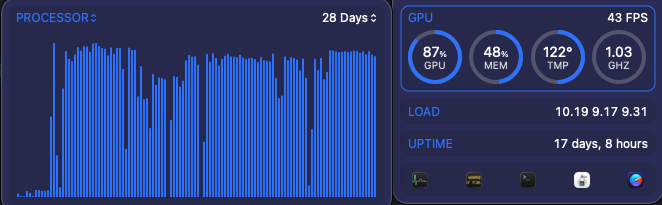
At this point of the journey my Mac Studio’s GPU has been camped out around 90% for nearly a month solid.

Why I Built Visualization Before the Model Was “Done”

At this point, I could train reasonably well, but I still didn’t fully trust the process as so many things had to be changed along the way.

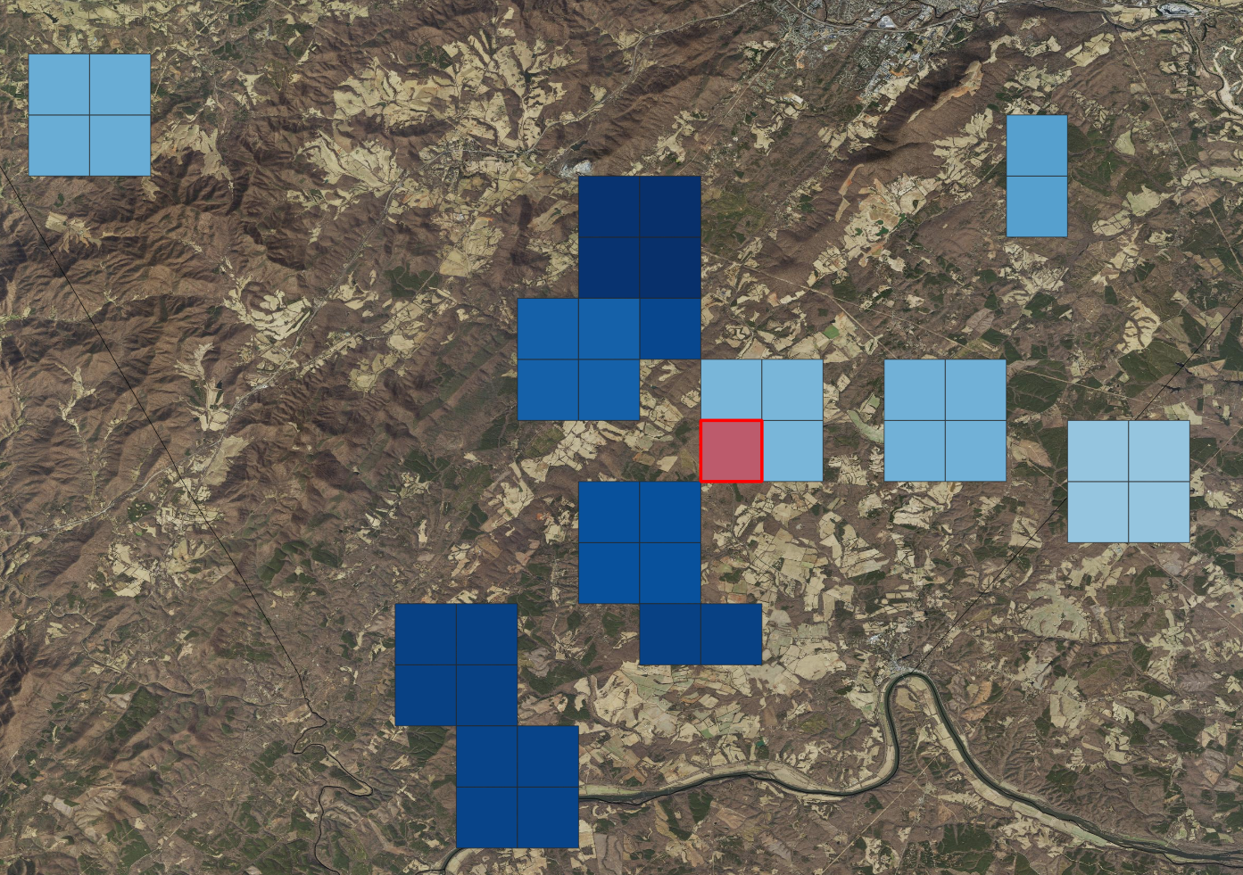
So I built visualization to see where the AI Model to Identify Ground in LiDAR has been learning.

Not pretty dashboards. Practical ones.

Tile footprints showing what the model has seen
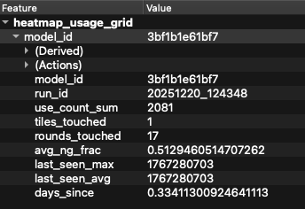
Heatmaps of usage and recency
Layers for first-seen tiles
Validation overlays

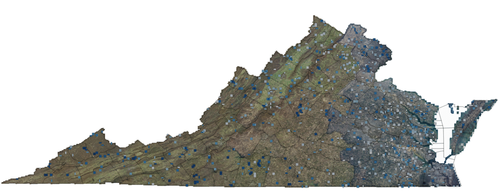
Exported as shapefiles, GeoJSON, and KML so I can open them in QGIS or Google Earth.

This let me answer questions like:

Is the model seeing the whole state?
Are some regions being oversampled?
Did validation tiles accidentally leak into training?

You can’t fix what you can’t see.

Tile footprints with index ramp of how much each foot print has been used

Where This Leaves the Model Right Now

At this point, the AI Model to Identify Ground in LiDAR is still early in its life and that matters.

Dense vegetation is still a challenge. Under heavy canopy, predictions can flip locally. That’s not surprising given how inconsistent ground truth is in those environments.

But the pipeline is now solid:

Training is incremental
Failures are visible
Sampling is intentional
Resume works
Caching is safe
Evaluation is meaningful

That’s the hard part.

Now, when the numbers move, I trust them.

And when they don’t, I know where to look.

What’s Next

In the next post, I’ll dig into specific failure cases:

When the model over-labels ground
When it becomes too conservative
How class weights and shard composition shift behavior
Why dense vegetation breaks naive ML approaches

This isn’t about chasing perfect metrics yet.

It’s about making sure that when improvement happens, it’s real.

For more geospatial workflows, see my post How I Turn Drone Data into Survey Deliverables. Come back to the blog for updates and behind-the-scenes insights. Also follow me on LinkedIn. If you need help with a project, I’m available, reach out and let’s talk.

How I’m Training an AI Model to Identify Ground in LiDAR, Part 3