How I’m Training an AI Model to Identify Ground in LiDAR – Inside the KPU-Net Workflow

LiDAR is one of the most powerful tools in GIS, Surveying, & Mapping, but one task has always been tricky:

Separating ground from everything else.
Trees, cars, buildings, utilities, and clutter, LiDAR sees it all, and so do we.

When training AI ground segmentation LiDAR models, traditional methods like PMF or cloth simulation still struggle in dense vegetation or complex terrain.

Over the past year I have been collaborating with Virginia Innovation Partnership Corporation and Virginia Commonwealth University on a research project which we recently published and it was presented at the 51st annual conference of the IEEE Industrial Electronics Society (IECON 2025) in Madrid, Spain. To continue on I am training my own deep learning ground classifier, based on the KPU-Net architecture — a model designed specifically for 3D point clouds.

Here’s a high-level look at how the system works and what’s happening under the hood while training on real USGS LiDAR data.

Step 1: Preparing USGS Files

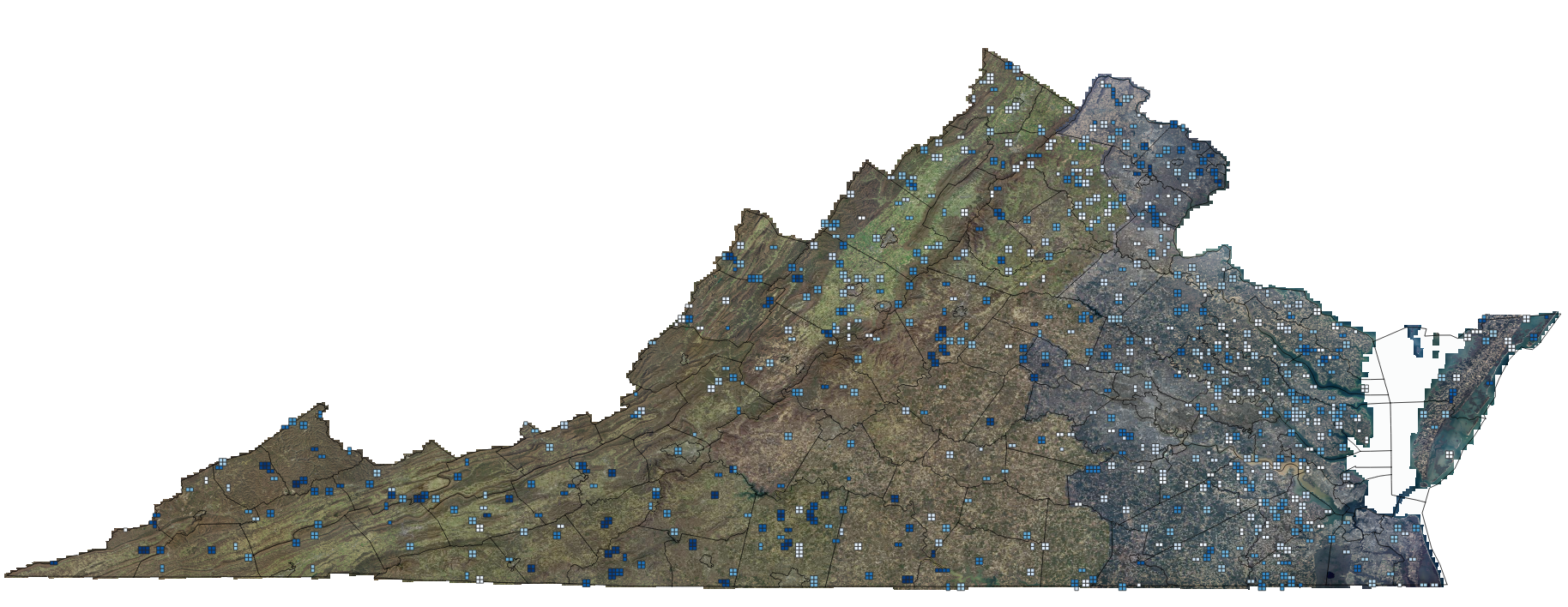
I’m grabbing USGS LiDAR data for this run, but all of our research was run using my data from the RiEGL VUX-1LR or RiEGL VQ480II platforms. Some of the USGS LiDAR tiles I’m using are 20–30 million points each. There is a Hidden Filesystem Problem With 1024-Point Tiles. One of the first challenges I knew I had to tackle was something most people never think about when working with LiDAR: your filesystem will choke if you generate too many tiny files.

Here’s why.

A typical USGS LiDAR tile can contain 20–30 million points.
If you split that into fixed-size chunks of 1024 points each, you get:

26,014,254 points / 1,024 ≈ 25,425 tiles

And if you store each tile as two files…

• tile_XXXX.npy (points)
• tile_XXXX_labels.npy (labels)

…that becomes:

25,425 tiles × 2 files ≈ 50,850 files

From a single LAZ file.

Now multiply that across the entire dataset I am training on:

• ~1,200 USGS LiDAR files (I am an overachiever, go big or go home)
• ~50,000 tile files per LAZ

You quickly end up with millions of tiny files, which creates serious problems:

• APFS/HFS+ starts slowing down
• directory listings become huge
• inode limits can be approached or exceeded
• backup tools and git repos crawl or fail
• training data loaders become inefficient

In short: storing tiles as individual .npy files does not scale.

This format keeps everything fast, tidy, and scalable.

The Training Data

Some of the USGS LiDAR tiles I’m using are 20–30 million points each.

Instead of splitting these into thousands of tiny files, I convert each LAZ into a single compressed “tile shard” that contains:

• fixed-size point tiles (1024–4096 points each)
• the point labels (ground / non-ground / ignore)
• the original point indices for reconstruction later

This format keeps everything fast, tidy, and scalable.

For this first experiment, I’m only using a single LiDAR tile to prove the workflow and architecture. Under the hood, that one LAS file is broken into thousands of fixed-size 3D tiles inside a single NPZ shard. So even though there’s just one source file on disk, the model is still training on millions of points.

At this stage, all training and evaluation is done on that tile. The goal here isn’t to claim a final accuracy number for all of Virginia, it’s to prove that the KPU-Net pipeline works end-to-end on real LiDAR data and to inspect the behavior of the model before I scale out to more tiles and more diverse terrain.

Step 2: Feeding Tiles Into the AI

The training loop reads these tiles in small batches — often just two tiles at a time — and sends them to the model. This is where training AI ground segmentation LiDAR models becomes powerful, because the system learns directly from labeled point tiles rather than hand‑tuned rules.

Each batch includes:

• XYZ coordinates
• ground labels from USGS
• masks for padded points
• and metadata so we can reassemble tiles later

This keeps training efficient even on consumer hardware like my Mac Studio.

Step 3: How KPU‑Net Learns Geometry for LiDAR Ground Segmentation

KPU-Net uses a technique called Kernel Point Convolution (KPConv), which works like a 3D version of image convolution.

It lets the model recognize geometric structures such as:

• flat ground
• berms and slopes
• tree canopies
• building edges
• asphalt vs vegetation transitions

Instead of hand-tuned rules, the model learns these patterns directly from the labeled point clouds.

Step 4: Loss, Regularization, and Class Balance

During training, the model outputs a probability for each point:

“How likely is it this point is ground?”

The console text below is a snapshot of the KPU-Net training process as it learns to identify ground points in a massive USGS LiDAR dataset. Each row represents a single epoch—a full pass through all the training tiles.

Here’s what the numbers mean:
regP / regF — small regularization penalties used to keep the model’s internal transformations stable
train_loss — the total error for the model during that epoch
seg — the main segmentation loss (how well the model predicts ground vs. non-ground)

david@Mac-Studio LiDARClassification % PYTHONPATH=. python -m kpunet train \ 
  --config configs/usgs_va.yaml \
  --train-tiles data/tiles/usgs_va \
  --output-dir models/kpunet \
  --batch-size 2

Epoch 1: train_loss=0.5120 seg=0.4328 regP=11.3803 regF=67.8241
Epoch 2: train_loss=0.3549 seg=0.3527 regP=1.3111 regF=0.9092
Epoch 3: train_loss=0.3273 seg=0.3265 regP=0.4997 regF=0.3503
Epoch 4: train_loss=0.3286 seg=0.3269 regP=0.9851 regF=0.6863
Epoch 5: train_loss=0.3198 seg=0.3189 regP=0.5744 regF=0.2928
Epoch 6: train_loss=0.3149 seg=0.3143 regP=0.4053 regF=0.1660
Epoch 7: train_loss=0.3140 seg=0.3134 regP=0.3274 regF=0.2834
Epoch 8: train_loss=0.3128 seg=0.3123 regP=0.3302 regF=0.1718
Epoch 9: train_loss=0.3140 seg=0.3133 regP=0.4140 regF=0.2739
Epoch 10: train_loss=0.3100 seg=0.3095 regP=0.3126 regF=0.1632
Epoch 11: train_loss=0.3106 seg=0.3101 regP=0.2753 regF=0.2225
Epoch 12: train_loss=0.3092 seg=0.3087 regP=0.3102 regF=0.2218
Epoch 13: train_loss=0.3088 seg=0.3084 regP=0.2812 regF=0.1590
Epoch 14: train_loss=0.3106 seg=0.3101 regP=0.3209 regF=0.2562
Epoch 15: train_loss=0.3083 seg=0.3077 regP=0.3534 regF=0.1635
Checkpoints saved to models/kpunet

What You’re Seeing Happen Over Time

• At Epoch 1, the model is still guessing and has a high segmentation error (seg=0.4350) and very large regularization terms.
• By Epochs 3–6, the segmentation loss drops sharply (0.33 → 0.31), showing the model is quickly learning the geometric patterns of USGS ground points.
• In Epochs 10–19, the loss values settle around 0.308–0.312, which is exactly what a stable training curve looks like.
• The regP and regF values shrink dramatically (from 70+ down to <1), meaning the learned transformations inside the network have become smooth and well-conditioned.

Its predictions are compared to the USGS labels, and the difference is used to update the model.

We add extra components to stabilize training:

• Class weights (because ground is usually <10% of points)
• Transformation regularization (keeps learned spatial transforms orthogonal)

Early epochs show large loss values as the model calibrates; then the loss settles into the ~0.30 range as learning stabilizes.

Validation of the Trained LiDAR Ground Segmentation Model

david@Mac-Studio LiDARClassification % PYTHONPATH=. python -m kpunet evaluate \
  --tiles data/tiles/usgs_va \
  --model models/kpunet/latest.pt

Accuracy: 0.7705, mIoU: 0.5013, acc_non_ground=0.7583, acc_ground=0.9011
Confusion matrix:
tensor([[18038863,  5748574],
              [  219890,  2002857]])

Interpretation (rows = true class, cols = predicted):

• Row 0: true non-ground
  • 18,038,863 correctly predicted non-ground
  • 5,748,574 incorrectly predicted ground (false positives)
• Row 1: true ground
  • 219,890 incorrectly predicted non-ground (false negatives)
  • 2,002,857 correctly predicted ground (true positives)

From that:

• Ground recall ≈ 90%
  → When a point is ground, the model finds it 9 times out of 10.
• Ground precision ≈ 26%
  → But among points the model calls “ground”, only about a quarter are truly ground.
• IoU non-ground ≈ 0.75
• IoU ground ≈ 0.25, giving mIoU ≈ 0.50

The model is great at not missing ground (high recall),
but currently over-labels ground (lots of false positives on buildings/roads/trees). For ground segmentation we are in a good place.

After training KPU-Net on a large USGS LiDAR tile, I evaluated the model on the same tiled dataset to get a first sanity check. The model achieved about 77% overall accuracy and a mean IoU of ~0.50 across ground and non-ground.

Looking at the confusion matrix, the network is very good at finding ground when it’s really there (around 90% recall for ground points), but it currently tends to over-predict ground in some areas, which lowers ground precision to the ~25% range. In other words, the model is conservative about missing ground (a good thing for DTMs), but still calls some buildings, roads, and other surfaces “ground” more often than we’d like.

This is exactly what I’d expect from a first pass trained on a single shard: the model has clearly learned what ground “looks like” in 3D, but still needs further tuning, better class balancing, and more diverse tiles before it will generalize cleanly across the full survey. I will continue to tune the model and pick up there in the next post.

Step 5: Using the Trained LiDAR Ground Segmentation Model

As soon as training completes, we save a checkpoint file containing the model’s learned parameters.

From there, we can:

• Run the model on new LAS/LAZ files
• Reconstruct a full classified point cloud
• Export a clean ground surface class
• Build DTMs, contours, and terrain models with fewer manual edits

This isn’t a toy, it’s a real ground segmentation engine that can plug into production workflows. I’ll show the progress and results of running the model in another post.

So what, why does this matter?

We’re entering an era where deep learning will become a standard part of GIS and survey-grade LiDAR processing workflows. I know we are on the cusp of the human in the loop stage of the workflow with eventual fully automated post processing.

Training your own models unlocks:

• repeatability
• cross-dataset robustness
• improved DTMs
• reduced editing time
• and new automation opportunities for drone and aircraft mapping

This project is just the beginning — and I’ll be sharing more results, comparisons, and tools as they evolve. Be sure to read the next post in this series.

For more geospatial workflows, see my post How I Turn Drone Data into Survey Deliverables. Come back to the blog for updates and behind-the-scenes insights. Also follow me on LinkedIn. If you need help with a project, reach out and let’s talk.